SMOTE explained for noobs – Synthetic Minority Over-sampling TEchnique line by line

What problem does SMOTE solve?

Machine learning algorithms learn poorly when one class dominates another. For example, imagine you are writing an algorithm to classify iris flowers by the length and width of the sepals. Your classifier learns from this data:

dat = iris[c(2, 9, 16, 23, 51:63),           c(1, 2, 5)]    > dat     Sepal.Length Sepal.Width    Species  2           4.9         3.0     setosa  9           4.4         2.9     setosa  16          5.7         4.4     setosa  23          4.6         3.6     setosa  51          7.0         3.2 versicolor  52          6.4         3.2 versicolor  53          6.9         3.1 versicolor  54          5.5         2.3 versicolor  55          6.5         2.8 versicolor  56          5.7         2.8 versicolor  57          6.3         3.3 versicolor  58          4.9         2.4 versicolor  59          6.6         2.9 versicolor  60          5.2         2.7 versicolor  61          5.0         2.0 versicolor  62          5.9         3.0 versicolor  63          6.0         2.2 versicolor  

You can easily see that the setosa flowers in red cluster in the top left and the green versicolor flowers in the bottom right. Unfortunately though, there are only 4 red flowers in the sample compared to 13 green flowers. All a machine learning algorithm sees is the domination of green flowers.

The domination of green flowers is even true in the range of values typical for red flowers. Let’s look at sepal length on the horizontal axis. Between the smallest red flower (sepal length = 4.4 cm) and the largest red flower (sepal length = 5.7 cm), there are 4 red flowers and 5 green flowers. It’s the same story on the vertical axis. All red flowers lie between sepal width values 2.9 cm and 4.4 cm. Nonetheless, there are more green flowers than red flowers in this range.

Based on the green domination, a machine learning algorithm could simply classify everything as green and still be correct 76% of the time.

There are 4 ways of addressing class imbalance problems like these:

• Synthesisis of new minority class instances
• Over-sampling of minority class
• Under-sampling of majority class
• tweak the cost function to make misclassification of minority instances more important than misclassification of majority instances

This blog post is exclusively about the first solution: synthesis of new minority class instances via SMOTE, as implemented in the R library smotefamily.

How does SMOTE resolve the class imbalance problem?

SMOTE synthesises new minority instances between existing (real) minority instances. Imagine that SMOTE draws lines between existing minority instances like this.

SMOTE then imagines new, synthetic minority instances somewhere on these lines.

library(smotefamily)    dat_plot = SMOTE(dat[,1:2],  # feature values                as.numeric(dat[,3]),  # class labels                K = 3, dup_size = 0)  # function parameters  

After synthesising new minority instances, the imbalance shrinks from 4 red versus 13 green to 12 red versus 13 green. Red flowers now dominate within the ranges typical for red flowers on both axes.

SMOTE function parameters explained

The SMOTE() of smotefamily takes two parameters: K and dup_size. In order to understand them, we need a bit more background on how SMOTE() works.

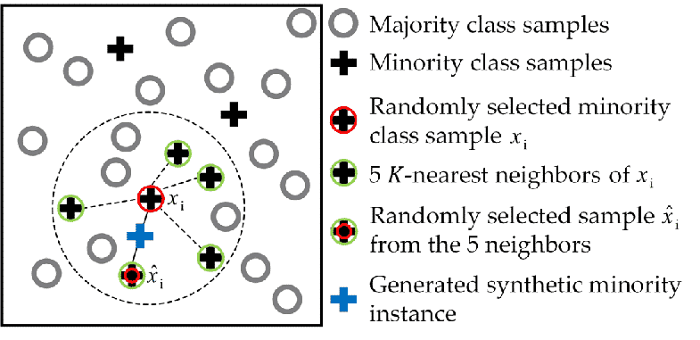
SMOTE() thinks from the perspective of existing minority instances and synthesises new instances at some distance from them towards one of their neighbours. Which neighbours are considered for each existing minority instance?

At K = 1 only the closest neighbour of the same class is considered. Let’s take the bottom right, red data point. By drawing a circle around the dot on the plot, we can easily see that the top left flower is its closest neighbour. Thus, at K = 1 SMOTE() synthesises a new minority instance on the line between these two dots when the bottom right flower is considered.

At K = 2 both the closest and the second closest neighbours are considered. For each new synthesis, a new one is randomly chosen between them.

In general, one might say that SMOTE() loops through the existing, real minority instance. At each loop iteration, one of the K closest minority class neighbours is chosen and a new minority instance is synthesised somewhere between the minority instance and that neighbour.

The dup_size parameter answers the question how many times SMOTE() should loop through the existing, real minority instances. Therefore at dup_size = 1 only 4 new data points are synthesised (1 for each existing minority instance). At dup_size = 200, 800 new data points get synthesised.

dup_size = 0 is a special case which uses the optimal number of minority class resuses in order to reach parity with the majority class.

SMOTE function code explained line by line

The SMOTE() function in the smotefamily library is explained easily enough. Siriseriwan Wacharasak wrote perfectly understandable code. Let me walk you through it.

SMOTE() takes four arguments:

• X = the feature values (e.g. sepal length and width)
• target = the class labels belonging to those feature values (e.g. iris species)
• K = how many of the closest neighbours are considered for synthesis
• dup_size = how many times existing data points get reused for synthesis (zero is a special case leading to balanced classes)

SMOTE <- function (X, target, K = 5, dup_size = 0) {  

First, the function checks the number of dimensions of feature space in ncD, the number of instances in each class in n_target, and the label of the minority class in classP.

ncD = ncol(X)  # check how many dimensions there are to the data  n_target = table(target)  # check how many instances of each class there are  classP = names(which.min(n_target))  # check the name of the minority class  

Next, the data (feature values and class labels) are split into minority and majority variables indicated by P and N respectively.

P_set = subset(X, target == names(which.min(n_target)))[sample(min(n_target)),]  # the minority feature values, in shuffled order  N_set = subset(X, target != names(which.min(n_target)))  # the majority feature values  P_class = rep(names(which.min(n_target)), nrow(P_set))  # class labels for minority instances  N_class = target[target != names(which.min(n_target))]  # class labels for majority instances  

The size of the minority and the majority classes are noted.

sizeP = nrow(P_set)  # the minority class sample size  sizeN = nrow(N_set)  # the majority class sample size  

Using the custom function knearest() from the smotefamily library, we get the indices of the K closest neighbours of each minority instance. In the table knear rows signify minority class instances and columns are the nearest neighbours in descending order (going from left to right). The number in each cell is the index of the neighbour.

knear = knearest(P_set, P_set, K)  # nearest neighbour indices  

Using yet another smotefamily custom function we learn how many times each data point should be reused as a starting point when generating new synthetic instances. The number of resuses is held by sum_dup. sum_dup is equivalent to dup_size for all integers except zero. In the zero case, the formula sum_dup = floor((2 * size_N - size_input)/size_P) is applied to find the optimal number for sum_dup to balance the classes.

There is no need to be intimidated by this formula. It determines how many synthetic instances we are away from balanced classes via (2*size_N - size_input). It then divides that number by how many existing, real minority instances we have via /P_set, given that sum_dup is the number of reuses of each minority instance. Whatever comes out of this is turned into an integer via floor().

sum_dup = n_dup_max(sizeP + sizeN, sizeP, sizeN, dup_size)  # smotefamily function  

And we are ready to loop over existing, real minority instances. The synthesised instances will be held in syn_dat.

syn_dat = NULL  # initialise the variable holding the synthetic data, no idea why this was not properly pre-allocated  for (i in 1:sizeP) {  # for each each minority instance  

In the loop we at first get the indices of the neighbours the currently considered minority instance will connect to. We sample with replacement from the K nearest neighbour indices and store the result in pair_idx.

  if (is.matrix(knear)) { #  if K > 1, i.e. if each minority sample has K nearest neighbours      pair_idx = knear[i, ceiling(runif(sum_dup) * K)] #  recall that knear holds the indices of K nearest neighbours, let's randomly sample from that with replacement    } else { #  if each minority sample only has one closest neighbour      pair_idx = rep(knear[i], sum_dup) #  get the nearest neighbour's index sum_dup number of times    }  

Where exactly between the currently considered minority instance of this loop iteration and its neighbours do we synthesise the new minority instance? The exact position is random and specified by g.

  g = runif(sum_dup)  # draw a random number between 0 and 1 sum_dup number of times, i.e. one number for each synthetic instance a minority data point will 'produce'  

We are nearly ready to synthesise. We just need matrices of the coordinates in feature space between which the new, synthesised instances will lie. P_i holds the coordinates of the minority sample of this loop iteration and Q_i holds the neighbours’ feature values.

  P_i = matrix(unlist(P_set[i, ]), sum_dup, ncD, byrow = TRUE)  # repeat the data of this minority sample a sum_dup number of times, i.e. once for each to be synthesised data point    Q_i = as.matrix(P_set[pair_idx, ])  # get the data of the neighbours of this minority sample, recall that neighbours are randomly chosen via pair_idx  

Having all the ingredients together, we can synthesise new instances. We take the distances between neighbour and currently considered minority sample coordinates in feature space via (Q_i - P_i). We reduce this distance by a factor g and add that to the coordinates of the currently considered minority sample P_i. The resulting synthetic minority instances with coordinates syn_i get addded to syn_dat.

  syn_i = P_i + g * (Q_i - P_i)  # create sum_dup samples between P_i, i.e. the coordinate of the real instance , and Q_i, i.e. the neighbours    syn_dat = rbind(syn_dat, syn_i)  # add the synthetic samples to the variable holding the totally of synthetic samples  }  

The rest of the SMOTE() function just organises the output without adding much to our understanding of the SMOTE algorithm. So, I put it here only for the sake of completeness.

P_set[, ncD + 1] = P_class  colnames(P_set) = c(colnames(X), "class")  N_set[, ncD + 1] = N_class  colnames(N_set) = c(colnames(X), "class")  rownames(syn_dat) = NULL  syn_dat = data.frame(syn_dat)  syn_dat[, ncD + 1] = rep(names(which.min(n_target)), nrow(syn_dat))  colnames(syn_dat) = c(colnames(X), "class")  NewD = rbind(P_set, syn_dat, N_set)  rownames(NewD) = NULL  D_result = list(data = NewD, syn_data = syn_dat, orig_N = N_set,                 orig_P = P_set, K = K, K_all = NULL, dup_size = sum_dup,                 outcast = NULL, eps = NULL, method = "SMOTE") #  put all information together which will be returned  class(D_result) = "gen_data" #  change the class of D_result to something called gen_data  return(D_result) #  return D-result when the function gets called  }  

If you want to access the original R script, including the plotting function, I used to make this blog post, look no further. It’s here.

Like this post? Share it with your followers or follow me on Twitter!